Making Estimates

Suppose you find yourself repeatedly conducting an experiment that sometimes fails and sometimes succeeds. Suppose further that each iteration of the experiment is identical, and random chance is the only difference between success and failure. This is analogous to repeatedly flipping a biased coin, a coin that shows heads with a probability that isn’t necessarily 0.5 as it is for a usual coin.

Let \(p\) be the unknown probability that your experiment succeeds. You would like to know the true value of \(p\), but the best you can do is estimate it based on the results of your experiments/coinflips.

An Estimator is a scheme for coming up with such an estimate \(x\), given a collection of observations. For example, say you’ve flipped your coin 10 times and heads has come up 7 times. An intuitive estimate for \(p\) would be \(x = 0.7\). This estimator is called the empirical mean. Now it’s possible that \(p\)’s true value is actually 0.7, but it could also one of infinitely many other possible values, in which case your estimate would not be perfectly accurate. In these cases it makes sense to measure the degree of accuracy of your estimate. There are different ways to measure this accuracy. One way is to compute the difference between your estimate and the true value, i.e. \(\lvert x - p \rvert\). We want this value to be 0, or at least as close to 0 as possible. Another measurement that’s more commonly seen in statistics is the function \((x - p)^2\). The idea of squaring the difference is to further penalize larger differences. These functions are called loss functions, and the two examples given are known as L1 loss and L2 loss respectively.

We can calculate the L2 loss: start with some underlying value for \(p\), generate sample observations using \(p\), use the estimator to generate an estimate \(x\), and then check the value \((x - p)^2\). The following code and graph shows the L2 loss using the empirical mean estimator for different values of \(p\).

import matplotlib
import matplotlib.pyplot as plt
import numpy as np


def estimate_empirical_mean(p, n):
    k = sum(np.random.random(size=n) < p)
    x = k / n
    return (x - p) ** 2

ps = np.arange(0.0, 1.0, 0.01)

fig, ax = plt.subplots()
N = 100
TRIALS = 1000
ax.plot(ps, [N * sum(estimate_empirical_mean(p, N) for _ in range(TRIALS)) / TRIALS for p in ps], color='red')

ax.set(xlabel='parameter p', ylabel='L2 Loss')
ax.grid()
plt.show()

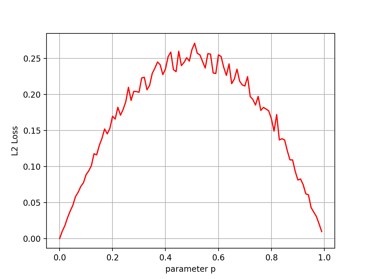
We see that our estimates are generally less accurate when \(p\) is closer to 0.5, and more accurate when \(p\) is close to 0 or 1. If you want to make guarantees about the accuracy of your estimator, you would use the worst case value, which here is around 0.25. The surprising thing I’d like to show in this post is that we can construct a new estimator that has a better guarantee than the empirical mean. Our new estimator will take the empirical mean estimate and move it slightly towards 0.5. This effectively “trades off” accuracy at the boundary values of \(p\) for accuracy around the middle.

Notice that this curve closely matches the parabola \(f(p) = p - p^2\). In fact if we were to run infinitely many trials, this curve would converge to that parabola exactly. Said more formally, the parabola \(p - p^2\) is the expected value of estimation error, denoted \(\mathbb{E}[(x - p)^2]\). Let’s work out the details to be sure.

Recall the formula for expected value, that it is the sum over all outcomes of the function value at that outcome times the probability of that outcome. In our setting, an outcome is observing some \(k\) heads after flipping a coin \(n\) times, where \(0 \leq k \leq n\) and \(x = \frac{k}{n}\). Then by linearity of expectation we expand:

We know that \(\mathbb{E}[k]\) is the expectation of the binomial distribution so its value is \(np\). \(\mathbb{E}[k^2]\) is harder to calculate, but fortunately we know that the variance of the binomial distribution is \(np(1-p)\) so we can use the formula for the variance \(\text{Var}[k] = \mathbb{E}[k^2] - \mathbb{E}[k]^2\) to find that \(\mathbb{E}[k^2] = np(1-p) + \mathbb{E}[k]^2 = np(1-p) + n^2p^2\). Now we can substitute and finish the algebra:

which exactly explains the graph! Whew, that was quite a bit of work.

As an aside, since I’m lazy, I’d prefer to not have to do all this tedious algebra. Fortunately the python package sympy can work out the details for us! Here is the same algebra as above, using sympy:

import sympy
p, n, k = sympy.symbols('p n k')
error = (k / n - p) ** 2
print(error.expand().subs(k ** 2, n * p * (1 - p) + n * n * p * p).subs(k, n * p).simplify())
>>> -p*(p - 1)/n

Now let’s embark on the adventure of coming up with a new estimator that moves the empirical mean towards 0.5. Two questions remain: how should it move the estimate, and by how much? We’ll tackle these two questions one at a time.

There are two normal ways I know of for moving a value \(x\) towards another value \(y\). The first, most common one, is linear interpolation: \((1-t)x + ty\) for some \(0 \leq t \leq 1\). \(t=0\) gives you \(x\), \(t=1\) gives you \(y\), and \(t=0.5\) gives you the midpoint between \(x\) and \(y\). In our problem setting, the estimate would like \((1-t)\frac{k}{n} + t\frac{1}{2}\), where we would need to pick a particular value for \(t\). In code we have:

def estimate_linear_interpolation(p, t, n):
    k = sum(np.random.random(size=n) < p)
    x = (1 - t) * k / n + t / 2
    return (x - p) ** 2

The second way I don’t know a name for, so I’d like to coin it as “hyperbolic interpolation”. If \(x=\frac{a}{b}\) and \(y=\frac{c}{d}\), then \(\frac{a+tc}{b+td}\) lies between \(x\) and \(y\) for \(0 \leq t < \infty\). You can imagine how adjusting \(t\) interpolates between the two values. This method is also inspired by Bayesian inference, as it matches the format of updating the Beta distribution, the conjugate prior for the binomial distribution. In our setting, this looks like \(\frac{k+t \cdot 1}{n+t \cdot 2}\). In code we have:

def estimate_hyperbolic_interpolation(p, t, n):
    k = sum(np.random.random(size=n) < p)
    x = (k + t) / (n + 2 * t)
    return (x - p) ** 2

Now it’s would normally be a lot of work to compute the optimal values of \(t\) in both of these interpolation formats, so we’ll use a trick to make things easier. Remember that we’re trading off accuracy at boundary values of \(p\) for accuracy around \(p=0.5\). In fact, an optimal value of \(t\) would yield a loss that’s a constant function of \(p\). The trick we’ll use is to set \(t\) to a value such that taking the derivative of the loss function with respect to \(p\) is 0. We can use sympy to do the dirty work, so we don’t have to.

def optimal_hyperbolic_interpolation():
    p, n, k, t = sympy.symbols('p n k t')
    error = ((k + t) / (n + 2 * t) - p) ** 2
    error = (
        error.expand()
        .subs(k ** 2, n * p * (1 - p) + n * n * p * p)
        .subs(k, n * p)
        .simplify()
    )
    d_dp = sympy.diff(error, p)
    return sympy.solve(d_dp, t)
>>> [sqrt(n)/2, -sqrt(n)/2]

def optimal_linear_interpolation():
    p, n, k, t = sympy.symbols('p n k t')
    error = ((1 - t) * k / n + t / 2 - p) ** 2
    error = (
        error.expand()
        .subs(k ** 2, n * p * (1 - p) + n * n * p * p)
        .subs(k, n * p)
        .simplify()
    )
    d_dp = sympy.diff(error, p)
    return sympy.solve(d_dp, t)
>>> [(sqrt(n) - 1)/(n - 1), -(sqrt(n) + 1)/(n - 1)]

Now the positive roots of each approach are the feasible ones, so we take \(t\) to be that value and graph the result.

import matplotlib
import matplotlib.pyplot as plt
import numpy as np


ps = np.arange(0.0, 1.0, 0.01)

fig, ax = plt.subplots()
N = 100
TRIALS = 1000
ax.plot(ps, [N * sum(estimate_empirical_mean(p, N) for _ in range(TRIALS)) / TRIALS for p in ps], color='red')

optimal_t = optimal_linear_interpolation()[0]  # the positive value
optimal_t = optimal_t.subs(list(optimal_t.free_symbols)[0], N)  # convert from sympy expression to numeric value
linear_interpolated_estimates = [N * sum(estimate_linear_interpolation(p, optimal_t, N) for _ in range(TRIALS)) / TRIALS for p in ps]
ax.plot(ps, linear_interpolated_estimates, color='green')

optimal_t = optimal_hyperbolic_interpolation()[1]  # the positive value
optimal_t = optimal_t.subs(list(optimal_t.free_symbols)[0], N)  # convert from sympy expression to numeric value
hyperbolic_interpolated_estimates = [N * sum(estimate_hyperbolic_interpolation(p, optimal_t, N) for _ in range(TRIALS)) / TRIALS for p in ps]
ax.plot(ps, hyperbolic_interpolated_estimates, color='blue')

ax.set(xlabel='parameter p', ylabel='L2 Loss')
ax.grid()
plt.show()

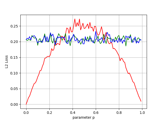
We did it! These modified estimators are mutually equivalent, and both have better worst case guarantees than the simple empirical mean.

QED! Until next time…

Sources: H. Steinhaus - The Problem of Estimation (https://projecteuclid.org/euclid.aoms/1177706876)