A Fast Solution to a Fibonacci Problem

Let’s try to find a fast solution to Project Euler’s Problem 2, which asks us to find the sum of the even-valued Fibonacci numbers that do not exceed four million. This is a beginner-level problem. After getting past the hump of realizing that Fibonacci numbers need to be cached/memoized/dynamic programming’d, a typical python solution might look like this:

import timeit

def P2(limit = 4*10**6):
    fibs = [1, 1]
    while fibs[-1] + fibs[-2] < limit:
        fibs.append(fibs[-1] + fibs[-2])
    return sum(x for x in fibs if x % 2 == 0)

num_trials, total_time = timeit.Timer('P2()', globals=globals()).autorange()
print(total_time / num_trials)
>>> 7.327787560000161e-06

Not bad! It already only takes 7.3μs, but let’s try to do better. As an amusing side note, the naive recursive solution without caching takes ~4s on my laptop, so we’re already over 500,000x faster.

Remove the list

Allocating a list is slow and unnecessary, since at any point we only need to access the last two values in the list. Let’s save only the last two values and see how it goes:

import timeit

def P2_no_list(limit = 4*10**6):
    previous_value, current_value, total = 1, 1, 0
    while current_value < limit:
        if current_value % 2 == 0:
            total += current_value
        previous_value, current_value = current_value, current_value + previous_value
    return total

num_trials, total_time = timeit.Timer('P2_no_list()', globals=globals()).autorange()
print(total_time / num_trials)
>>> 2.8692420399999996e-06

About three times faster!

Remove the odd valued terms

Take a look at where the even values are situated in the Fibonacci sequence:

1, 1, 2, 3, 5, 8, 13, 21, 34, …

It seems like every third term is even. This isn’t a coincidence. Since the Fibonacci sequence is a linear recurrence, the sequence of remainders when dividing each term by any fixed number will be periodic (homework: prove this!). With this recurrence \(F_n = F_{n-1} + F_{n-2}\), the pattern of odd and even numbers will be Odd, Odd, Even, Odd, Odd, Even, Odd, Odd, Even, ..., since Odd + Odd = Even and Odd + Even = Odd.

Using that information, we can try to come up with a way to compute the even terms while ignoring the odd terms completely. Expanding out the definition of the sequence:

Now if we let \(G_n := F_{3n}\), we get \(G_n = 4G_{n-1} + G_{n-2}\) with \(G_0 = 0\) and \(G_1 = 2\), a perfectly good recurrence that exactly captures the even terms in the fibonacci sequence!

import timeit

def P2_no_odd_terms(limit = 4*10**6):
    previous_value, current_value, total = 0, 2, 0
    while current_value < limit:
        total += current_value
        previous_value, current_value = current_value, 4 * current_value + previous_value
    return total

num_trials, total_time = timeit.Timer('P2_no_odd_terms()', globals=globals()).autorange()
print(total_time / num_trials)
>>> 1.1106692099999993e-06

Another almost 3x speedup!

Remove the accumulator

There is an identity \(\sum_{i=0}^n F_i = F_{n+2} - 1\) that expresses the sum of fibonacci numbers in terms of a single value. Let’s prove this, and then maybe we can come up with a similar formula for the even terms:

By telescoping the sum on the right hand side. So we should be able to do the same with \(G_n\):

Where the last substitution uses the recurrence definition of \(G_n\). So we can rewrite our function without using an accumulator at all!

import timeit

def P2_no_accumulator(limit = 4*10**6):
    previous_value, current_value = 0, 2
    while current_value < limit:
        previous_value, current_value = current_value, (4 * current_value) + previous_value
    return (previous_value + current_value - 2) >> 2

num_trials, total_time = timeit.Timer('P2_no_accumulator()', globals=globals()).autorange()
print(total_time / num_trials)
>>> 9.136303600025712e-07

Another 1.2x speedup.

On this note, there’s another Fibonacci identity that can save us some time. Notice that we’re adding every third term, each of which is equal to the sum of the two preceding terms. This means that adding all the terms should give us double the result we want. E.g.:

2 + 8 + 34 = 44

1 + 1 + 2 + 3 + 5 + 8 + 13 + 21 + 34 = 88 = 2 × 44

Now we can leverage the formula we saw before for summing usual Fibonacci sequences: \(\sum_{i=0}^n G_i = \sum_{i=0}^n F_{3i} = \frac{1}{2} \sum_{i=0}^{3n} F_i = \frac{1}{2} (F_{3n+2} - 1)\) We can calculate \(H_n = F_{3n+2}\) using the same recurrence for \(G_n\), but now with initial conditions \(H_0 = F_2 = 1\) and \(H_1 = F_5 = 5\). Now our function looks like:

import timeit

def P2_no_accumulator_2(limit = 4*10**6):
    previous_value, current_value = 1, 5
    while current_value < limit:
        previous_value, current_value = current_value, (4 * current_value) + previous_value
    return current_value >> 1

num_trials, total_time = timeit.Timer('P2_no_accumulator_2()', globals=globals()).autorange()
print(total_time / num_trials)
>>> 8.271025819994975e-07

A mild 1.1x speedup.

Remove the loop?

The hardest thing to tackle is removing the loop entirely, which is why we save it for last. Now that our problem amounts to calculating one or two terms in the Fibonacci sequence, why not use Binet’s Formula to calculate it directly instead of looping? Well for one, that formula requires knowing which index in the sequence we want to calculate, whereas we’re looking for the largest term that doesn’t exceed a specified limit. There are two options I see here: calculate the index directly first using a logarithm, or use something like Interpolation Search to find the right term by trial and error. A problem with the logarithm approach is that it uses floating point arithmetic, so it is succeptible to rounding errors for sufficiently large limits. In my testing, at around limit=\(10^{14}\) this approach started giving wrong answers, making it overall pretty undesirable. Omitting some of the algebra details, my attempt looks like this:

import timeit

def P2_logarithm(limit=4*10**6):
    index = int(math.log(limit * math.sqrt(5), 2 + math.sqrt(5))) + 1
    return round(((2 + math.sqrt(5))**index - 1) / (5 + math.sqrt(5)))

num_trials, total_time = timeit.Timer('P2_logarithm()', globals=globals()).autorange()
print(total_time / num_trials)
>>> 8.342724520043703e-07

Slightly slower, and untrustworthy for larger limits. It is the most concise solution though, which at least makes us look clever :).

For interpolation search, first we need to understand a matrix identity using Fibonacci numbers:

This can be seen by just multiplying the matrices through and using the recurrence relation of the Fibonacci numbers. What this means is that we can calculate \(F_n\) by calculating \(A^n\) and looking at its entries. This is fortunate because we can use repeated squaring to calculate \(A^n\) in \(O(\log(n))\) operations, hopefully saving us some time. Since we don’t know exactly what \(n\) is ahead of time, our algorithm will need to repeatedly square powers of \(A\) until exceeding the limit, and then back off and repeat. This will take \(O(\log(n)^2)\) operations, which should still eventually be faster than the previous algorithm which took \(O(n)\). Finally, after finding the largest \(F_n\) smaller than the limit, we’ll need to do a bit of case work to find the largest \(F_{3k+2}\) smaller than the limit. This looks like:

import numpy as np
import timeit

def P2_squaring(limit = 4*10**6):
  A = np.array([[1, 1], [1, 0]])
  while A[0][0] < limit:
    B = np.array([[1, 1], [1, 0]])
    while True:
      B_squared = B @ B
      if (A @ B_squared)[0][1] > limit:
        break
      B = B_squared
    A = A @ B
  if A[0][0] % 2 == 0:
    return (2 * A[0][0] + A[0][1] - 1) // 2
  elif A[0][1] % 2 == 0:
    return (A[0][0] + A[0][1] - 1) // 2
  else:
    return (A[0][0] - 1) // 2

num_trials, total_time = timeit.Timer('P2_squaring()', globals=globals()).autorange()
print(total_time / num_trials)
>>> 2.4940721999155356e-05

Much slower, because numpy has a bunch of overhead for multiplying matrices. Now don’t look at the following code, which is the same algorithm with matrix multiplication done barehand, because it’s atrocious:

def P2_squaring_optimized(limit = 4*10**6):
  a, b, c = 1, 1, 0
  while a < limit:
    x, y, z = 1, 1, 0
    while True:
      tx, ty, tz = x * x + y * y, x * y + y * z, y * y + z * z
      if a * ty + b * tz > limit:
        break
      x, y, z = tx, ty, tz
    a, b, c = a * x + b * y, a * y + b * z, b * y + c * z
  if a % 2 == 0:
    return a + (b >> 1)
  elif b % 2 == 0:
    return (a + b) >> 1
  else:
    return a >> 1

num_trials, total_time = timeit.Timer('P2_squaring_optimized()', globals=globals()).autorange()
print(total_time / num_trials)
>>>2.9668219599989244e-06

So we get an order of magnitude speedup, but still 3x slower than our previous attempts. This is because while we’ve improved the asymptotic complexity, our constant overhead has become worse, and the actual \(n\) is small. What we would expect is that as we increase the limit, this squaring function will eventually get faster than our previous attempts. Let’s check the runtime at a few different limits, plotted on a log-log plot:

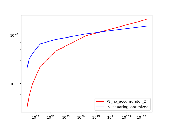
It looks like our new algorithm eventually gets faster for limits above \(10^{80}\), so it takes quite a while. Not what we hoped for, but at least now we know.

Closing thoughts

We got about a 9x overall speedup from the naive dynamic programming solution for this problem by using a variety of clever ideas and tools. Of course we could get a massive speedup by just not using Python, but the purpose of this post was to demonstrate conceptual optimizations so that’s less important. There’s also some beautiful theory using generating functions that provides a deeper understanding to a lot of this stuff. We chose to do things in a more elementary way here to be more direct.

Until next time…