How Accurate is Your Rating?

You’re playing a competitive online team game. You notice that your teammates seem to be underperforming, and can’t help but wonder why. Are they boosted? Are they just having a bad game? Has their rating not converged yet? Has their rating been artificially inflated because they happened to win several of their most recent games? In this post we analyze and quantify the likelihood of this last possibility.

Skill Ratings

Skill rating systems like Elo are commonly used in games to represent each player’s skill level with a number. A rating is considered accurate if it can be used, together with various formulas, to accurately predict the outcomes of games. Before a player has played any games, they are given a provisional rating which will likely not be very accurate. As they play more games, the system updates its estimates, and eventually converges on a rating that is fairly close to optimal. With the Elo system, this convergence period generally lasts for several dozen games. More modern systems like Glicko and TrueSkill use more sophisticated statistical techniques, and they can converge in half as many games as Elo or less.

Once a player’s rating has converged on their true skill, the rating itself will continue to fluctuate around that value as more games are played. The question we address in this post is: what are the magnitudes of these fluctuations? On average, how accurate is the rating of a player who has passed the convergence period?

How Accurate is Your Rating?

To state our question formally, we’ll need some assumptions. We’ll use the Elo system, which gives us a simple way to sample outcomes of games between two players by using the prescribed formula. We also assume that at any rating the matchmaker will give you an opponent that is perfectly matched for you. This is often pretty close to the truth in online video games, especially more popular games with larger player populations.

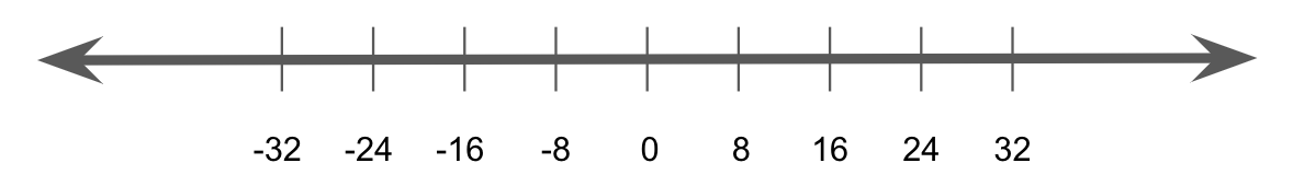
With this setup, a player’s rating over time can be modelled as a random walk around their true rating. With a typical K-factor of 16 and perfect matchmaking, a win will increase the rating by exactly 8 points, and a loss will decrease it by exactly 8 points. Therefore, letting \(r_0\) be the true rating, the random walk has discrete support over the state set \(\{r_0 + 8k, k \in \mathbb{Z}\}\). For simplicity we’ll identify these states with the integers, so ratings of \(\{r_0 - 16, r_0 - 8, r_0, r_0 + 8, r_0 + 16\}\) will be represented by states \(\{-2, -1, 0, 1, 2\}\).

The probabilities associated with moving left and right in this random walk depend on which state we’re in, which is different from the prototypical unbiased setting for random walks. This makes sense for rating systems though; it should be more likely that you take a step towards your true rating than away from it. Let \(A\) be the matrix of transition probabilities where \(A_{i,j}\) is the probability of transitioning from state \(i\) to state \(j\). Then by the Elo formula,

The second case here is a number slightly above \(0.5\) for moving towards your true rating, and the third case is slightly below \(0.5\) for moving away from your true rating.

The Markov Chain associated to this random walk has a steady state distribution. The formalized question is now: for the Markov Chain with transition probabilities described above, what is the average distance from the \(0\) state, when averaged over its steady state distribution? Put another way, what is the Mean Absolute Error (MAE) of a player’s converged rating?

Monte Carlo Solution

The simplest approach to measuring the average error is using Monte Carlo simulation. Essentially we simulate many games using our model, collect the results, and empirically measure the average error. The code and plots for this approach look like this:

import collections
import random
import matplotlib.pyplot as plt

K = 16

def expected_winrate(a, b):
    return 1 / (1 + 10**((b - a) / 400))

def rating_delta(a, b, a_win):
    return K * (a_win - expected_winrate(a, b))

def monte_carlo(steps):
    true_rating = 0
    visits = collections.defaultdict(int)
    current_rating = true_rating

    for _ in range(steps):
        visits[current_rating] += 1
        a_win = random.random() < expected_winrate(true_rating, current_rating)
        current_rating += rating_delta(current_rating, current_rating, a_win)

    return {k: v / steps for k, v in visits.items()}

def plot(visits, **kwargs):
    plt.plot(*zip(*sorted(visits.items())), **kwargs)
    mae = sum(abs(k)*v for k, v in visits.items())
    print(f"Mean Average Error: {mae}")

def show_plots():
    plt.legend()
    plt.xlabel('rating')
    plt.ylabel('probability')
    plt.show()

>>> plot(monte_carlo(10**3), color='red')
Mean Average Error: 26.64000000000002

>>> plot(monte_carlo(10**5), color='blue')
Mean Average Error: 29.72592000000098

>>> plot(monte_carlo(10**7), color='green')
Mean Average Error: 29.845985600157935

>>> show_plots()

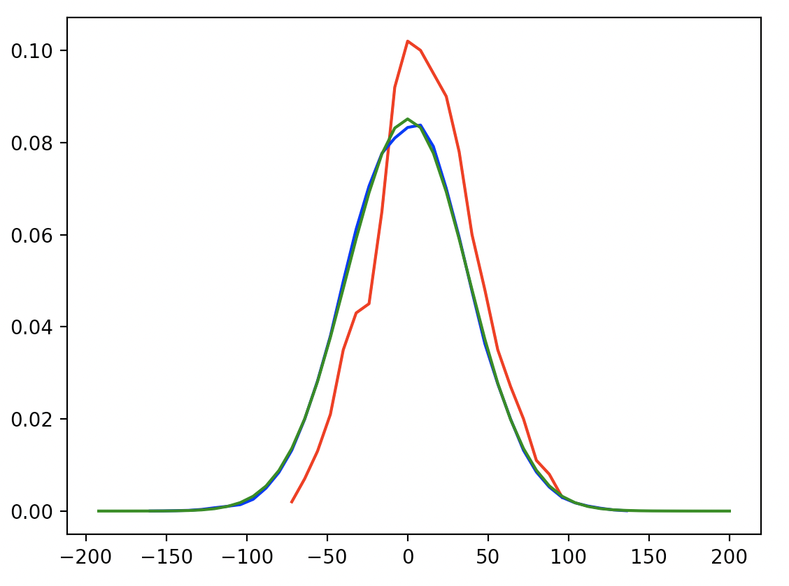
There will be a slight bias towards smaller MAE since this simulation starts exactly at the true rating, but it seems to be dominated by simulation variance because the MAE shown is slightly increasing as the number of simulation steps increase.

So there you have it, on average your rating will be about 30 points away from what it should be. All things considered, that’s not too far off! With the same procedure we can also look at some quantiles: the 50th percentile error is 24, the 80th is 40, and the 95th is 56.

Analytic Solution

The Monte Carlo solution is decent, but it’d be great to get a more accurate answer, and ideally an exact answer. We’re trying to find the mean absolute error, which we could calculate directly if we knew the steady state distribution of the Markov Chain we constructed. The standard technique to find such a steady state distribution uses linear algebra to solve for \(Av=v\), but our Markov Chain has infinitely many states, so that won’t work. Fortunately we can still make progress by using some clever techniques.

Proposition

Let \(M\) be a finite-state Markov Chain on \(n\) states, with transition matrix \(A\), and steady state distribution \(S\). Now let \(G(V, E)\) be the undirected graph induced by \(M\), where \(V = S\) and \(E = \{(u, v) \mid \ u, v \in V, u \neq v, A_{u,v} \neq 0\ \textit{or} \ A_{v,u} \neq 0 \}\). If \(G\) is acyclic, then:

Proof

We can assume \(G\) is connected without loss of generality, as otherwise we could apply same logic to each of the connected components without any issues. Now we proceed by induction on \(\mid M \mid\), the number of states in \(M\). If \(\mid M \mid\) \(= 1\), \(G\) has no edges so the proposition is vacuously true. Otherwise \(G\) has some vertex \(x\) with degree 1, that is connected to another vertex \(y\). Now by the definition of a steady state, \(S(x) = \sum_{y} A_{y, x} S(y)\), but in this case the right hand side only has two nonzero terms:

Since \(A\) is a stochastic matrix, \(\sum_{y} A_{x,y} = 1\), so \(A_{x,x} = 1 - A_{x,y}\), and we get:

Therefore the proposition holds at the edge \((x, y)\). By the inductive hypothesis it also holds for all edges in \(G \setminus \{x\}\) which is also acyclic. Since \(x\) has degree 1, this covers all the edges in \(G\), so the proposition holds, QED.

Now we’ll assume that a steady state exists. Let \(S^*\) be the steady state distribution of \(M'\), i.e. a function that assigns probabilities to states in \(M'\) such that \(\sum_{x \in M'} S^*(x) = 1\). Then let \(S\) be another function with the same signature defined by \(S(x) = \frac{S^*(x)}{S^*(0)}\) be an unnormalized function of the same sort, scaled so that \(S(0) = 1\).

We’ll use this construction to iteratively solve for \(S(1)\), and then \(S(2)\), and so on. Notice that \(M\) satisfies the assumptions of the proposition: it is a line, so it is certainly acyclic. Technically \(M\) has infinitely many states and the proposition was for finitely many states, but if we squint a little and apply the technique anyways, we can still make progress. So applying the proposition gives:

It makes sense for \(S(1)\) to be a bit under \(2\) (while \(S(0) = 1\)), because recall we sandwiched two states into one for \(S(1)\), each which will have a bit less weight than \(S(0)\) which did not come from two states. For clarity, let’s call \(\alpha = 10^{\left( \frac{8}{400} \right)}\). Then \(S(1) = 1 + \alpha^{-1}\). Similarly let’s calculate \(S(2)\):

…

Now we can expand the consecutive ratios all the way back to \(S(1)\):

And finally collapse them, noting that \(\frac{1 + \alpha^{-k}}{1 + \alpha^k} = \alpha^{-k}\):

What a beautiful simplification! Now let’s clean up and summarize what we’ve done. We solved for \(S(k)\) for all \(k \in \mathbb{N}\), but remember that \(S\) is only proportional to the steady state distribution \(S^*\). To renormalize, we need to divide by the sum \(T = \sum_{k \in \mathbb{N}} S(k)\) to find the scaled version of \(S\) that is an actual probability distribution. This is an infinite sum, but at first glance it resembles a geometric series so we might hope to use an identity like \(\sum_{k \in \mathbb{N}} \alpha^k = \frac{1}{1-\alpha}\) to find a closed form. Unfortunately, \(T\) is actually a Theta function that is known to have no closed form. So close, yet so far.

At least we can approximate \(T\) astronomically more efficiently than the Monte Carlo approach, with the following code:

alpha = 10**(8/400)

def T(upper_bound):
    result = 1
    for k in range(1, upper_bound):
        result += alpha**(-k*(k+1)/2) + alpha**(-k*(k-1)/2)
    return result

>>> print(T(1000))
11.748085322402272

>>> print(T(40))
11.748085322402272

As we can see, for values of \(k\) above 40, the cumulative value of \(T\) changes by less than machine epsilon and is therefore imperceptible. Now let’s sanity check our math by comparing it to the Monte Carlo approach:

def S(k):
    return (alpha**(-k*(k+1)/2) + alpha**(-k*(k-1)/2)) / T(40)

def analytic(window):
    return {8 * i: S(i) / 2 for i in range(-window, window + 1)}

>>> plot(monte_carlo(10**7), color='blue', label='monte carlo')
Mean Average Error: 29.818871999999995

>>> plot(analytic(40), color='red', label='analytic')
Mean Average Error: 29.80184236053276

>>> show_plots()

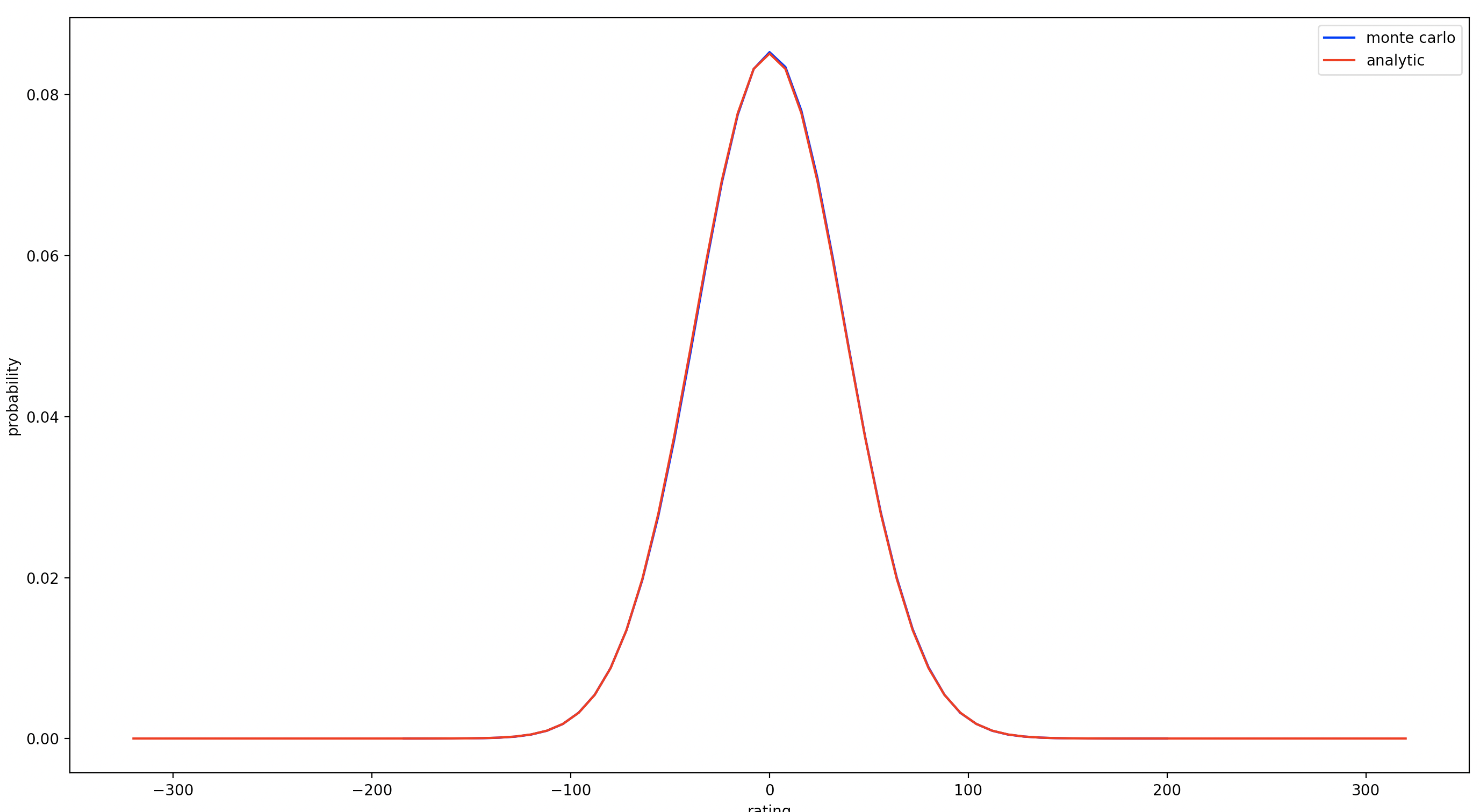
So it looks like the Monte Carlo estimate is ~0.017 off, and it runs in 7s compared to 200μs for the analytic solution (3000x speedup).

In summary, we found that on average, ratings prescribed by the Elo system will be inaccurate by around 30 points. We first calculated this with a crude but direct Monte Carlo simulation, and then calculated it again with a more complicated but accurate analytic derivation. I hope you learned something! Until next time…