You’ve been playing a competitive online game for a while. You notice that rating is relatively stagnant, but you’d like to reach the next level, and then take a break. This is a common engagement pattern for players, as seen in e.g. Chess or Dota 2 Ideally you’d like to do so in a way that doesn’t require you to get better at the game, because that seems hard. In this post we’ll investigate how many games it’ll take for you to hit that next level purely by random chance.
Random Walks of Ratings
We saw in a previous post that in the Elo rating system, ratings will randomly fluctuate around their intended value. On average they’ll be about 30 points off, but we can also try to calculate a different question: if I want to reach, say, 50 rating points above my true value, how many games will I expect to have to play for that to happen by random chance?
In stochastic process theory, this is called a hitting time problem. We want to calculate \(\tau(0, n)\), the time starting from \(0\) to hit a point \(n\) steps in the positive direction. As in the previous post, we’ll calculate this first using a fast-and-dirty Monte Carlo method, and then try to solve it with more sophisticated tools.
Monte Carlo Simulation
Calculating \(\tau(0, n)\) with Monte Carlo simulation essentially amounts to converting the stochastic process into code, running it for a bunch of trials, and averaging the results. This is what that looks like:
import random

def p_win(n):
    return 1 / (1 + 10 ** (n / 50))

def p_loss(n):
    return 1 - p_win(n)

def monte_carlo_hitting_time(n, num_trials=100):
    total_steps = 0
    for _ in range(num_trials):
        steps = 0
        current_position = 0
        while current_position < n:
            current_position += 1 if random.random() < p_win(current_position) else -1
            steps += 1
        total_steps += steps
    return total_steps / num_trials
Because we’re working with the Elo rating system with a standard \(k\)-factor of 16, the value of \(n\) represents the number of net wins that we’d like to reach. Each win is worth 8 rating points, so to hit 50 rating points above our true skill, we’d need 7 net wins.
>>> monte_carlo_hitting_time(7)
214.94
>>> monte_carlo_hitting_time(7)
192.84
>>> monte_carlo_hitting_time(7)
177.02
>>> monte_carlo_hitting_time(7, num_trials=100_000)
200.27782
>>> monte_carlo_hitting_time(7, num_trials=100_000)
200.41436
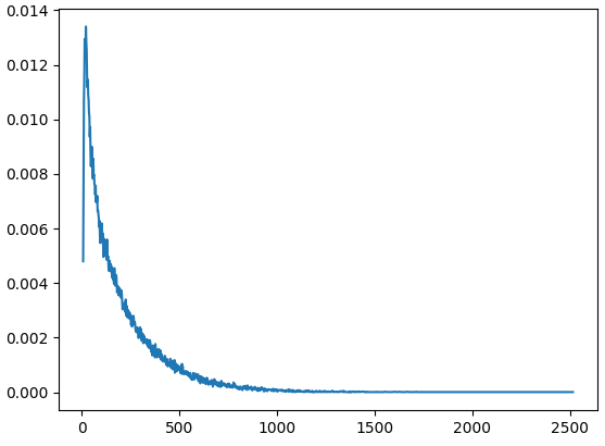
Notice that this method produces pretty significant variance for 100 trials, but works well enough for 100,000 trials. This runs in about 9 seconds on my computer. 200 is a lot of games to just get 7 net wins though! Let plot the distribution of how many games this actually takes:
import collections
import matplotlib.pyplot as plt

def monte_carlo_hitting_time_distribution(n, num_trials=100):
    steps_counter = collections.Counter()
    for _ in range(num_trials):
        steps = 0
        current_position = 0
        while current_position < n:
            current_position += 1 if random.random() < p_win(current_position) else -1
            steps += 1
        steps_counter[steps] += 1
    return steps_counter

num_trials = 100000
steps_distribution = monte_carlo_hitting_time_distribution(7, num_trials)
steps_distribution = sorted([(k, v / num_trials) for k, v in steps_distribution.items()])
plt.plot(*list(zip(*steps_distribution)))
plt.show()
Faster and more accurate computation
Now we try to simplify the problem to see if we can solve it faster and more accurately. Borrowing the notation from the previous post, let \(S^*\) be the Markov Chain representing the dynamics of one’s rating changing over time. For a generic Markov Chain the formula for \(\tau(x, y)\), the expected time to first reach state \(y\) starting from state \(x\), is:
\[\tau(x, y) = \begin{cases} 0 &\ \text{if } x = y \\ 1 + \sum_{z \in S^*} A_{x,z} \tau(z, y) & \text{ otherwise } \\ \end{cases}\]We’re working with a specific type of Markov Chain, so we use a simpler formula. If we’re starting at state \(0\) and want to reach state \(n\), we’ll need to reach state \(n-1\) first, before then proceeding to \(n\). So \(\tau(0, n) = \tau(0, n-1) + \tau(n-1, n)\). Now, before reaching \(n-1\) we must reach \(n-2\), and so on, which gives the formula:
\[\tau(0, n) = \sum_{k=0}^{n-1} \tau(k, k+1)\]Now it remains to reduce \(\tau(k, k+1)\) further. For this we can use the fact that the only nonzero transitions out of state \(k\) are \(k-1\) and \(k+1\). Referencing the first formula:
\[\begin{align*} \tau(k, k+1) &= 1 + \sum_{z \in S^*} A_{x, z} \tau(z, y) \\ &= 1 + A_{k, k+1} \tau(k+1, k+1) + A_{k, k-1} \tau(k-1, k+1) \\ &= 1 + A_{k, k-1} (\tau(k-1, k) + \tau(k, k+1)) \\ (1 - A_{k, k-1}) \tau(k, k+1) &= 1 + A_{k, k-1} \tau(k-1, k) \\ \tau(k, k+1) &= \frac{1 + A_{k, k-1} \tau(k-1, k)}{(1 - A_{k, k-1})} \end{align*}\]At this point, we’ve established a recursive formula for \(\tau(k, k+1)\). To test the formula, we can implement it in code and see if the results agree with our Monte Carlo simulation. Notice that we have to put a limit on the recursion, since our states include all of \(\mathbb{Z}\), so if we ran this formula as described the program would never terminate. When the limit is a sufficiently large negative number, the probability of taking a step in the negative direction - aka losing a game - is negligible so we can round it to 0.
def recursive_hitting_time(n, limit):
    return sum(recursive_stepping_time(k, limit) for k in range(n))

def recursive_stepping_time(k, limit):
    # time to get from state k to k+1
    if k == limit:
        return 1
    else:
        return (1 + p_loss(k) * recursive_stepping_time(k - 1, limit)) / p_win(k)

>>> recursive_hitting_time(7, limit=-1000)
200.01670103012418
>>> recursive_hitting_time(7, limit=-40)
200.01670103012418
For limits below -40 we can see that the error is less than machine epsilon. Our answer agrees with the Monte Carlo answer, so we can be pretty confident that our derivation was correct. Also, this code runs in less than 1 millisecond, so we got a speedup of over 9000 over the Monte Carlo method. It’s good progress, but ideally we could express the answer directly in a closed form. We can in fact do better if we get our hands dirty and make a sacrifice to the algebra gods:
\[\begin{align*} \tau(k, k+1) &= \frac{1 + A_{k, k-1} \tau(k-1, k)}{(1 - A_{k, k-1})} \\ \tau(k, k+1) &= \frac{1}{(1 - A_{k, k-1})} + \frac{A_{k, k-1}}{(1 - A_{k, k-1})} \tau(k-1, k) \\ \end{align*}\]Recall that \(A_{k, k-1} = \frac{1}{1 + 10^{-k/50}}\), so letting \(\alpha = 10^{1/50}\) we get
\[\frac{1}{(1 - A_{k, k-1})} = 1 + \alpha^k\]and
\[\frac{A_{k, k-1}}{(1 - A_{k, k-1})} = \alpha^k\]Using this we now unroll the recursive formula, with the base case assumption that \(\tau(-L, -L+1) \approx 1\) for a sufficiently large limit \(L\).
\[\begin{align*} \tau(k, k+1) &= 1 + \alpha^k + \alpha^k \tau(k-1, k) \\ &= 1 + \alpha^k + \alpha^k (1 + \alpha^{k-1} + \alpha^{k-1} \tau(k-2, k-1)) \\ &= 1 + \alpha^k + \alpha^k + \alpha^{k + (k-1)} + \alpha^{k + (k-1)} + \alpha^{k + (k-1) + (k-2)} + \cdots + 1 \\ &= 1 + 2 \left( \alpha^k + \alpha^{k + (k-1)} + \alpha^{k + (k-1) + \cdots} + 1 \right) \\ &= 1 + 2 \left( \sum_{m=0}^L \alpha^{(\sum_{i=k-m}^k i)} \right) \\ &= 1 + 2 \left( \sum_{m=1}^L \alpha^{(m (k + 1) - \frac{m(m+1)}{2})} \right) \\ &= 1 + 2 \left( \sum_{m=1}^L \alpha^{(m k - \frac{(m - 1)m}{2})} \right) \end{align*}\]Again we check our work with code:
def iterative_hitting_time(n, limit):
    return sum(iterative_stepping_time(k, limit) for k in range(n))

def iterative_stepping_time(k, limit):
    alpha = 10 ** (1 / 50)
    return 1 + 2 * sum(alpha ** (m * k - ((m - 1) * m) / 2) for m in range(1, -limit))

>>> iterative_hitting_time(7, limit=-40)
200.0167010300768
We now have a formula that sums \(O(n^2)\) terms. With even more work we can reduce this to \(O(n)\):
\[\begin{align*} \tau(0, n) &= \sum_{k=0}^{n-1} \tau(k, k+1) \\ &= \sum_{k=0}^{n-1} \left(1 + 2 \left( \sum_{m=1}^L \alpha^{(m k - \frac{(m - 1)m}{2})} \right) \right) \\ &= n + 2 \left( \sum_{k=0}^{n-1} \sum_{m=1}^L \alpha^{(m k - \frac{(m - 1)m}{2})} \right) \\ &= n + 2 \left( \sum_{m=1}^L \sum_{k=0}^{n-1} \alpha^{(m k - \frac{(m - 1)m}{2})} \right) \\ &= n + 2 \left( \sum_{m=1}^L \alpha^{- \frac{(m - 1)m}{2}}\sum_{k=0}^{n-1} (\alpha^{m})^{k} \right) \\ &= n + 2 \left( \sum_{m=1}^L \alpha^{- \frac{(m - 1)m}{2}} \frac{\alpha^{mn} - 1}{\alpha^m - 1} \right) \\ \end{align*}\]def analytic_hitting_time(n, limit):
return n + 2 * sum(a ** (- (m * (m - 1)) / 2) * (a ** (m * n) - 1) / (a ** m - 1) for m in range(1, -limit))
>>> analytic_hitting_time(7, limit=-40)
200.0167010300768
Unfortunately for the same reason as the previous post, the sum of a theta function has no closed form so we won’t be able to reduce it further, but this is still significant progress over the previous versions. On my computer recursive_hitting_time(7, limit=-40) runs in 263μs, iterative_hitting_time(7, limit=-40) runs in 80.6μs, and analytic_hitting_time(7, limit=-40) runs in 25μs. Not bad for a more accurate and 360,000x faster calculation than the Monte Carlo simulation.
Conclusion
We found that if you try to reach a rating 50 points above where you belong, it will take you 200 games on average, but after 64 games you’ll have succeeded with 50% probability. We first calculated this directly via Monte Carlo simulation, and then calculated it again with a more accurate analytic derivation. I hope you learned something! Until next time…